
짜리몽땅 매거진
[ML] 텍스트 벡터화하고 LDA 토픽모델링하기 본문
정성데이터를 가공할 때, 텍스트 데이터에서 단어를 추출해야할 때 등 여러 케이스에서 자연어처리(NLP)를 해야하는 경우가 많다. 이때 초반에 진행해야하면서 기초적이지만 중요한 부분이 바로 '벡터화'이다.
텍스트 벡터화는 텍스트 데이터를 수치 데이터로 변환하는 과정으로, 머신러닝 모델이 텍스트를 이해하고 처리할 수 있게 하는 중요한 단계이다. 그 중 가장 널리 알려진 Count Vectorizer와 TFIDF Vectorizer를 다루고자 한다.
1. Count Vectorizer
CountVectorizer는 텍스트 데이터에서 단어의 빈도를 세어 벡터로 변환하는 클래스이다.
from sklearn.feature_extraction.text import CountVectorizer

# 예시 리스트
corpus= [
    'This is the first corpus',
    'This corpus is the second corpus',
    'And this corpus is the third one',
    'Is this the first corpus?'
]

# CountVectorizer
cv=CountVectorizer()

# 문서 벡터화
X =cv.fit_transform(corpus)

# 변환 결과 출력
print('corpus 사용한 피처 : ',cv.get_feature_names_out())
print('----')
print('매트릭스 확인 : ',X.toarray())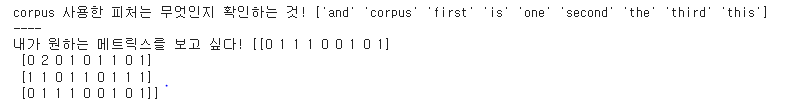
2. TF-IDF Vectorizer
TfidfVectorizer는 단어의 빈도(TF)와 역문서 빈도(IDF)를 결합하여 단어의 중요도를 평가하는 클래스이다.
from sklearn.feature_extraction.text import TfidfVectorizer

# 예시 리스트
corpus= [
    'This is the first corpus',
    'This corpus is the second corpus',
    'And this corpus is the third one',
    'Is this the first corpus?'
]

# TFIDF 벡터화
vectorizer = TfidfVectorizer()

X=vectorizer.fit_transform(corpus)

# 변환 결과 출력
print('corpus 사용한 피처 :',vectorizer.get_feature_names_out())
print('----')
print('매트릭스 확인 :',X.toarray())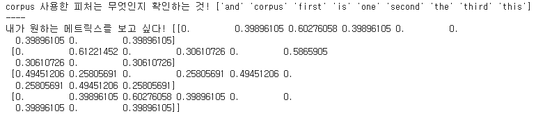
그렇다면 이제 벡터화된 데이터를 기반으로 유사도를 측정해 LDA(토픽모델링)까지 진행해보자.
유사도는 두 텍스트 데이터가 얼마나 비슷한지를 측정하는 값으로, 텍스트 간의 유사도를 계산하면 텍스트 분류, 정보 검색, 추천 시스템, 감성 분석 등에 활용할 수 있다. 그 중 가장 널리 쓰이는 코사인 유사도에 대해 살펴보자.
코사인 유사도 (Cosine Similarity)는 두 벡터 간의 각도를 기반으로 유사도를 측정하는 방법으로, 벡터의 크기보다는 방향을 고려하여 계산하며, 값은 -1에서 1 사이의 범위를 가지는데, 텍스트 유사도에서 0~1 범위로 주로 사용된다.
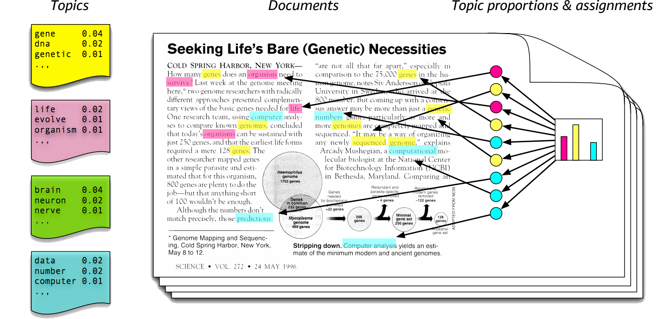
LDA 토픽 모델링은 는 문서 내에 존재하는 단어들을 기반으로 잠재 주제(토픽)를 식별하는 모델이다. 각 문서는 여러 토픽의 혼합으로 구성되어 있다고 가정하고, 문서 내 단어 출현 빈도를 분석하여 특정 단어들이 어떤 토픽에 속할 확률이 높은지를 계산한다.
영화 리뷰 샘플 데이터셋을 활용해 벡터화부터 유사도 측정, 토픽모델링까지 실습해보자.
import pandas as pd

# 영화 리뷰 데이터 불러오기
df=pd.read_csv('movie_rv.csv')
df_sp=df.iloc[:50000]

import re
from konlpy.tag import Okt

# Okt 형태소 분석기 생성
okt =Okt()
텍스트를 형태소 별로 처리하기 위해 Okt 형태소 분석기를 먼저 생성한다.
# 전처리 함수
def preprocess_text(text):
#문자열 확인하고, 아니면 빈 문자열 반환
if not isinstance(text,str):
return ''
#특수문자 제거
text=re.sub(r'[^ㄱ-ㅎㅏ-ㅣ가-힣\s]','',text)
#형태소로 분석을 통해 추출 (명사만 추출)
nouns=okt.nouns(text)
return ' '.join(nouns)
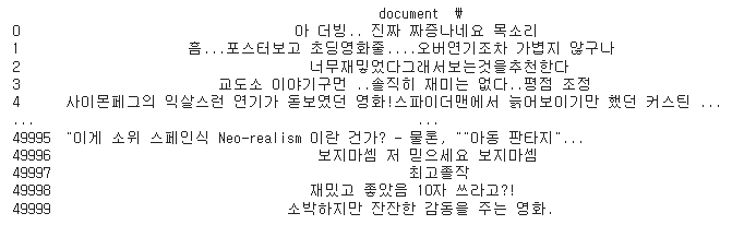
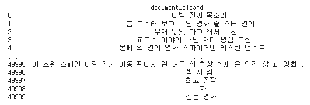
df_sp['document_cleand']=df_sp['document'].apply(preprocess_text)
print(df_sp[['document','document_cleand']])
이렇게 특수문자 제거, 명사 추출 등의 함수를 작성한 뒤, 전처리된 값을 확인하면 아래와 같다.
이제 앞서 배운 벡터화를 사용해 수치 데이터로 변환하고, 유사도를 측정해보자.
# CountVectorizer
cv=CountVectorizer()
X_cv_count=cv.fit_transform(df_sp['document_cleand'])

# tfidf
tfidf = TfidfVectorizer()
X_tfidf_count=tfidf.fit_transform(df_sp['document_cleand'])

# cosine_similarities
from sklearn.metrics.pairwise import cosine_similarity

cos_sim_count = cosine_similarity(X_cv_count)
cos_sim_tfidf = cosine_similarity(X_tfidf_count)

# 코사인 유사도를 통해 리뷰 10개 정도 추려서 리뷰와 코사인 유사도가 같은 Top3 리뷰를 출력

num_rvs = 10
for i in range(num_rvs):
    #cv
    simliar_indices_count = cos_sim_count[i].argsort()[::-1][1:11]
    similar_reviews_count = [(cos_sim_count[i][j], df_sp['document'][j]) for j in simliar_indices_count]

    #tfidf
    simliar_indices_tfidf = cos_sim_tfidf[i].argsort()[::-1][1:4]
    similar_reviews_tfidf = [(cos_sim_tfidf[i][j], df_sp['document'][j]) for j in simliar_indices_tfidf]

    print(f"\n Original Review {i+1}: {df_sp['document'][i]}")
    print("\n Top 3 similar reviews using countvectorizer:")
    for sim_score, reviews in similar_reviews_count:
        print(f"Similarity :{sim_score:.3f}, Reviews:{reviews}")

    print("\n Top 3 similar reviews using Tfidf:")
    for sim_score, reviews in similar_reviews_tfidf:
        print(f"Similarity :{sim_score:.3f}, Reviews:{reviews}")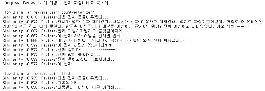
from sklearn.decomposition import LatentDirichletAllocation

# LDA모델 학습
lda=LatentDirichletAllocation(n_components = 2, random_state=111)

lda.fit(X_cv_count)

# 상위 몇 개 단어를 가지고 올 것인가?
n_top_words = 10

def print_top_words(model, feature_name, n_top_words):
    for topic_idx, topic in enumerate(model.components_):
        print(f"Topic {topic_idx}:")
        print(" ".join([feature_name[i] for i in topic.argsort()[:-n_top_words-1:-1]]))

tf_feature_names=cv.get_feature_names_out()
print_top_words(lda, tf_feature_names, n_top_words)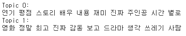
이렇게 벡터화, 유사도 측정, 토픽모델링까지 진행했는데, 원하는 토픽 주제는 분석가 정할 수 있다. 위 예시에서는 2개의 토픽을 정하는데, 이 토픽은 어떤 특정 값이 아니라 계산해서 유사하다고 판단되는 토픽들을 묶어서 보여주는 것이다.
'Data > Machine Learning' 카테고리의 다른 글
| [ML] 유저이탈 예측하기 (0) | 2025.01.04 |
|---|---|
| [ML] AutoML_TPOT으로 최적 모델 찾기 (1) | 2024.10.29 |
| [ML] Sweetviz와 Pipeline으로 모델링하기 (0) | 2024.10.29 |
| [ML] 데이터 샘플링 (0) | 2024.10.25 |
| [ML] 데이터 변환 (1) | 2024.08.19 |


